
I was asked by some friends to share what I use for figuring out how many samples are needed, usually for setup or creating protocols. I have posted this in the Download section of sigmakatadojo.com for anyone who would like it. The secret (it’s no secret) is that a sample of one is not valid, and there’s a distinction between ad-hoc design of experiments and actual testing.
In the wonderful world of product development where adrenaline runs freely and breakthrough inventions are like Easter eggs it can be easy to build a plywood and ball-bearing prototype, get it to work and declare success – running headlong into production. I watched a smart and talented designer do just that with millions of dollars of investor’s money, only to find long term failure. He has multiple patents, none of them meet requirements. Why? He didn’t test his work – he made a trial design, got the answers he wanted and ran fast forward. I worked with a company that had developed a special case for long-haul shipment of their very expensive product. They expected to make two – maybe three – of these cases in the next 10 years. Do they need to have multiple units to test? No. Do they need to do multiple tests? Oh, yes.
There are some statistical values to consider in setting sample sizes. These are dependent on whether the result is attribute – which is to say good vs. bad, pass vs. fail – or continuous. Continuous means values of measurement – weight, length, temperature, etc. Then the next consideration is the confidence level needed in the results and the reliability of the measurement. Since confidence level has to do with measurement it obviously is not a factor in attribute results. Attribute results lean on confidence of the results, of course, but also in the reliability of the data – will it repeat one test after another. Let’s think about attribute first.
For attribute results, figuring the number of samples you need to collect uses the equation: SS = ln(alpha)/ln(reliability). Before we go further, I didn’t create the math. I just use it. I worked with an MIT graduate who loved to derive everything – that’s not me. The “alpha” here is the percent remaining after you remove your confidence level – the amount that might be wrong (the chance of rejecting the null hypothesis when it is actually true). So if you need a confidence of 95% the alpha, the part that might be wrong, is 5%. Reliability is referring to how often the results will repeat. If you ask for a reliability of 90% that means you expect the results to land within the alpha range nine times out of ten. One time out of ten it will fall outside the alpha and that is acceptable. Remember, we’re talking attribute here – right or wrong, pass or fail. Let’s say you have a process that makes pregnancy tests. You want to be able to tell folks that the results are 99% reliable, and you have a solid process so the company will support a 90% confidence. If the process was known to have odd results the company might push for higher confidence in the test results, but since the historic data shows really consistent results, a sample built around a 90% confidence is accepted. The sample size from this would be ln(0.01)/ln(0.9) = 44. Forty-four tests with perfect results is a pass. There is no margin for bad results. One bad result in 44 means the test failed.
For continuous data, measurement, the equation (again – not mine) uses a thing called a double-tailed Z chart. This chart converts the alpha – the part that can go wrong – into a Z sigma factor. A Z factor of 1.96 is indicating an alpha of 5%. The path to connect 5% to 1.96 works like this: the chart is double-tailed, so the alpha is double or representing the full range – i.e. alpha of 5% means +/-2.5%. So looking at the Z chart for an alpha of 5% means looking for a Z for 2.5% or 0.025. Here’s the chart:
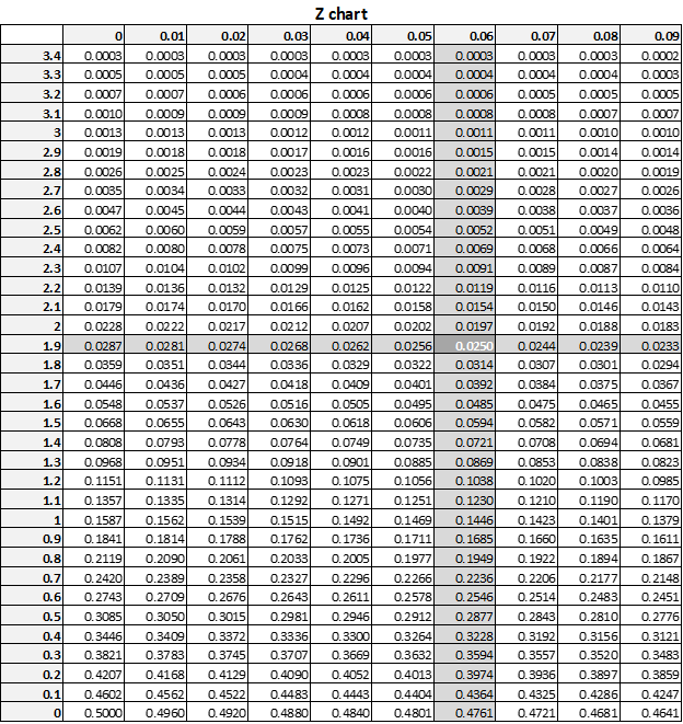
This chart converts your alpha to your Z value – which is needed shortly.
Next step is to determine your margin of error. Traditionally this is determined by taking the amount you can vary, like +/- 5, and dividing by the total measurement, say 127. This example would be e = 5/127 = .04. Last step is to find the standard deviation of the process, called sigma. Then plug these values into the equation SS = (Z^2 * sigma^2) / e^2.
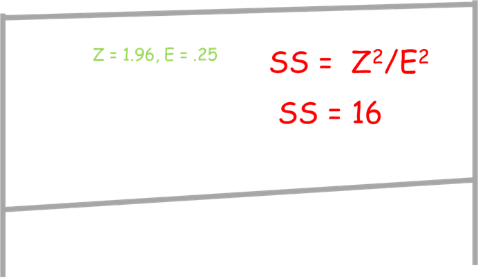
Since I have always found that it is better not to overthink a thing, I reconsidered the math. What I found is, since you need to get samples to determine the standard deviation anyway, if you set your margin of error as a percent of the standard deviation you compress the work and math to this:
Let E = sigma * %error; SS = Z^2 / E^2
I will say right now that many a serious statistician will disagree with this approach. The subtle nuances of statistics just can’t be simplified in this way, and they are right. On the other hand, having used this approach for over a decade and tested it’s ability to meet the needs of production, this does work for processes that are in reasonable statistical control. If you use this approach it is important to use the standard deviation from the approach so you can tell if the output is in control.
The simplicity and elegance of using this instead of the standard means you can determine the sample size for a setup quickly based on this:
Standard Deviation is not out of control, so using 50% of a standard deviation, currently less than 1/3 of the required tolerance, is more than adequate. Therefore the sample size SS = 1.96^2 / 0.5^2 = 16.
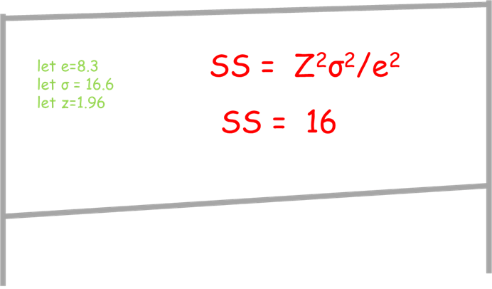
Because the serious statisticians are resistant, let’s run a proof. Assume the sample size is needed to make sure a peen hammer is striking consistently, the impact needs to be between 800 and 1000 lbf with a duration less than .002 seconds. The mean is 900 lbf, the duration needs to be under 2ms. We need to set the mean impact of the hammer, and since we want +/-100 lbf and we expect 3 sigma performance we can say the margin of error is lbf, or one-half of 3 sigma of 50 lbf = 100 / (3/.5) = 8.3. Using the equation referenced SS = Z^2/E^2 and Z = 1.96, E = .5. Using the standard equation and collecting the data to determine a standard deviation of the samples (16) we find the standard deviation for a sample setup to be 15, nice and repeatable – well within the 16.6 value. Plugging into the stock equation of SS = (Z^2 sigma^2) / e^2 where e is the margin of error.
You do not need to know sigma to apply this, but you do need to know if the process is under control.
This is to say that 16 samples is enough to tell you if the setup is within +/- 50% of the standard deviation, or since the standard deviation is known to be less than 1/3 of the tolerance the setup is within +/- 17% of dead nominal. Many control charts begin in this range or greater.
I have included a vanilla procedure in the download section for my friends who would like to use this in their companies. I strongly recommend they write a protocol to evaluate the data, since the algebraic conversion is not widely recognized. I have run a protocol against this several times over the past ten years, and have had one outlier – which is statistically expected – and was not repeated.
Thanks for letting me share my experiences!
